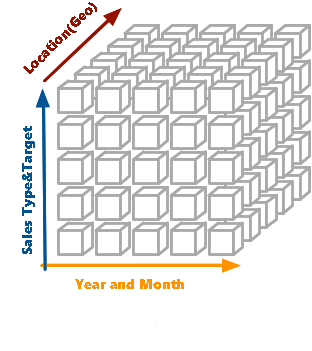
Definition of OLAP cube: Refer
Usage of OLAP cube for Sales MIS in Kea: We used cubes to implement Sales MIS module in our product Kea. Process of the implementation is explained in the following sections:
As for an example, we may have the following dimensions in a warehouse for keeping master and transaction sales data.

- Zonal Data (Location)
- Product Data(Master Key)
- Customer Master(Master Key)
- Year
- Month
- Sales(Primary & Secondary).
That layout (a 5D “cube”) would allow queries to be easily performed to customers and that may have different types of sales reports throughout the year/ specific month & year.
All of those key parts would just point to a single sales figure of month in a specific month in a specific year in a specific location (Team, Zone, State & etc…) for a specific customer.
An example on how to access that data. Let’s say we want to see how all sales patterns changed on a monthly basis, averaged over all the years. You would do this to see which customers generated the most revenue for you at specific times of the year so you could; for example, target your advertizing at them in the month or so before then.
We can use the customer master and Product to extract information, effectively “collapsing” the location, year and month dimensions (in other words, sum up the sales figures for those three dimensions to get a two-dimensional result, customers vs. month).
Below example has three dimensions (LocationMaster, customer, product) and one fact (sales). So a typical Kimball star would look like:

A dimension (table) is a look-up table for properties of objects that rarely change. Product, customer and LocationMaster may change some of their properties (attributes), but they rarely do. Fact table captures interactions between these objects. At the intersection of dimensions Month, Year, sales, product and customer lies a measure SalesAmount. Note how easy is to aggregate (sum) the sales amount by month, by year, by product, by brand, by city, by country.
Facts and Measures:
Fact is most detailed information that can be measured.
Example of a fact might be Sales, a target, TA%, Growth%. We can measure:

- Sales :Primary Sales, Secondary Sales, Closing
- Target :Location target , quantity target
- YTD :Financial budget, financial year sales
- Growth &TA:Calculation based on above facts.
Those measurable properties, such as amount, target and growth are called measures.
We are mostly interested in summarized view: “what were the overall sales?”, “what are the sales achieved on particular duration?” or “how many persons are there?” Those computed values are called aggregates or aggregated measures.
Facts might have multiple measures or they might even have none.
Concept Hierarchies:
We might be interested in sales per year, then per month for particular year; products can be grouped by categories and subcategories; location (Geo) might be defined by country, country might have multiple cities… Those are concept hierarchies of dimensions.
Hierarchy has multiple levels and there might be various hierarchical views of any dimension. For example split by year, quarter, month and day wise. From technical perspective we might associate an attribute with a dimension. Depending on the modeling method a dimension might be composed of just one attribute or multiple attributes grouped by hierarchies.
Slicing and Dicing:
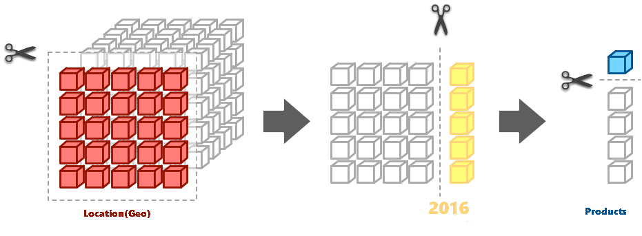
We have a data cube full of facts, how can we explore the data? We can slice the cube!
Example 1:
We have a report which shows the yearly based sales performance of a particular product. But we want to see it in a monthly/Quarterly wise. So we can use slicing and dicing technique to drill down to monthly level.
Example 2:
Slicing – Total number of units sold for a product over a specific time frame.
Dicing – overall sales for specific product, produced by different specific time in specific Location (zone, region, Country).
